『 Attention Is All You Need. 2017. 』
Transformer 모델은 현재 Vision, NLP 등 분야를 가리지 않고 사용되고 있다. 그만큼 "Attention is all you need" 논문은 현재까지도 많은 영향을 끼치고 있고 최근 인공지능이 이렇게 빨리 발전할 수 있는 원동력이 되었다고 생각한다. Transformer 모델에 대해서는 이전에 개념공부를 한 적이 있지만, 논문을 뜯어보며 리뷰를 했던 것은 아니기에 이제서야 진행해보려 한다.

Transformer 개념 정리
https://rahites.tistory.com/66
[D&A Deep Session] 9차시 - 15. Attention, Transformer
## 지금까지 Sequence data를 처리하는데 사용한 RNN계열의 알고리즘은 t-1번째 hidden state와 t번째 input data를 활용하여 recurrent model을 만들었다. 하지만 Sequence가 진행됨에 따라 Sequence 앞에 존재하던 원
rahites.tistory.com
0. Abstract
- 지금 시퀀스 변환 모델은 Encoder와 Decoder를 포함하는 복잡한 순환 or 합성곱 신경망에 기반을 둔다.
- 본 논문에서는 Attention 매커니즘만을 사용하고 순환 or 합성곱 방식을 완전히 제거한 새로운 Transformer 아키텍처를 제안한다.
1. Introduction
지금까지는 RNN, LSTM, GRU 모델들이 sequence modeling이나 transduction problem에서 SOTA를 기록해왔다. 하지만 RNN 계열의 recurrent 모델은 일반적으로 입력 및 출력 시퀀스의 position을 순차적으로 계산하기 때문에 문장을 한번에 처리하지 못한다는 단점을 지닌다. 즉 메모리 제약문제로 인해 Parallelization이 불가능하기 때문에 길이기 긴 시퀀스에서 치명적인 단점으로 작용하는 것이다.
이를 극복하기 위한 Factorization이나 Conditional Computation 방법 등이 연구되었지만 Sequential Computation의 근본적인 한계가 남아있는 것이 사실이다. 따라서 본 논문에서는 Attention 매커니즘만을 사용하여 그 한계를 극복한다. Attention 매커니즘의 입력 또는 출력 사이에서 거리에 관계없이 Dependency를 모델링할 수 있다는 특징을 살리고, 이전까지의 연구에서 Attention과 Recurrent Network를 같이 사용한 것과 달리 본 논문에서는 Attention 매커니즘만을 사용한 Transformer 모델을 소개한다.
※ Transduction
: 하나의 문자열을 다른 문자열로 변환하는 것
https://dos-tacos.github.io/translation/transductive-learning
Sequence prediction (1): transductive learning
다양한 분야에서 쓰이고 있는 ‘Transduction’ 개념이 특히 언어학, 시퀀스 예측 분야에서는 어떻게 사용되는지 알아봅니다.
dos-tacos.github.io
2. Background
Sequential Computation을 줄이려는 시도는 Extended Neural GPU, ByteNet, ConvS2S 에서도 이루어졌다. 이 모델들은 CNN을 basic building block으로 사용하고, 모든 input과 output position에 대한 hidden representation을 병렬로 계산한다는 특징을 가진다.
Self-attention(intra-attention)은 sequence의 representation을 계산하기 위해 하나의 sequence에서 서로 다른 position을 연결한다. 또한 reading comprehension, abstractive summarization, textual entailment 등의 task에서 성공적으로 사용하였다. (하나의 시퀀스가 있을 때 시퀀스의 단어가 서로에게 가중치를 부여하는 작업)
※ Attention Mechanism
15-01 어텐션 메커니즘 (Attention Mechanism)
앞서 배운 seq2seq 모델은 **인코더**에서 입력 시퀀스를 컨텍스트 벡터라는 하나의 고정된 크기의 벡터 표현으로 압축하고, **디코더**는 이 컨텍스트 벡터를 통해서 출력 …
wikidocs.net
End to End는 sequence aligned recurrence보다 recurrent attention 매커니즘에 기반하고 간단한 문답이나 언어 모델링 task에서 좋은 성능을 가진다.
Transformer는 Sequence aligned된 RNN이나 Convolution을 사용하지 않고 self-attention만을 사용한 최초의 transduction 모델이다.
※ Alignment
https://dos-tacos.github.io/concept/alignment-in-rnn/
Sequence prediction(2): RNN에서의 alignment 의미와 seq-to-seq 모델
RNN에서 alignment의 의미와 기존 모델의 어려움을 극복하기 위해 제안되었던 Seq2seq 모델에 대해 알아봅니다.
dos-tacos.github.io
3. Model Architecture
3.1. Encoder and Decoder stacks
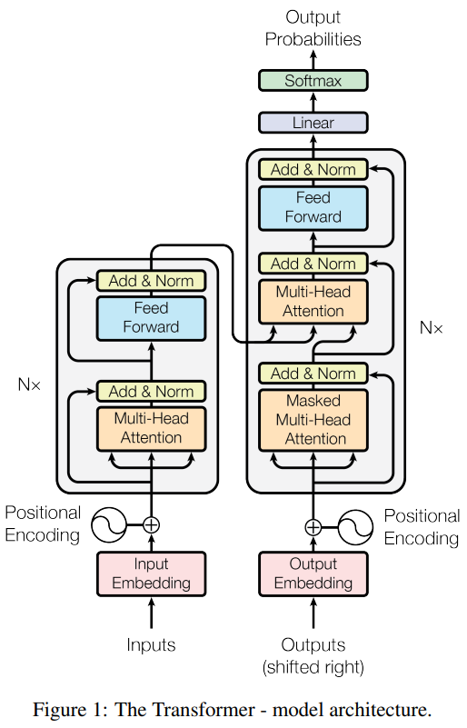
Encoder
- 6개의 동일한 layer로 구성
- 각 layer는 2개의 sub-layer를 가짐 (첫번째는 multi-head self-attention이고 두번째는 position-wise fully connected feed-forward network)
- 각각의 sub-layer마다 layer normalization을 마친 뒤 residual connection을 진행
- residual connection을 용이하게 하기 위해 embedding layer과 모든 sub-layer들은 512의 차원을 가진다.
($d_{model} = 512$)
1. 임베딩 벡터에 positional encoding 값을 더해 인코더에 입력
2. Input으로 query, key, value를 계산해 Multi-Head attention에 입력
3. Add&Norm에서 잔차 연결과 정규화 진행
4. Feed Forward층에서 선형변환과 활성화 함수 적용
5. Add&Norm에서 잔차 연결과 정규화 진행
6. Encoder의 output 배출
※ Residual Connection (잔차 연결)
: 상위 layer의 gradient 값이 변하지 않을 채로 하위 layer에 전달되는 것으로 layer를 거칠수록 gradient가 사라지는 gradient vanishing 문제를 완화
https://arxiv.org/abs/1603.05027
Identity Mappings in Deep Residual Networks
Deep residual networks have emerged as a family of extremely deep architectures showing compelling accuracy and nice convergence behaviors. In this paper, we analyze the propagation formulations behind the residual building blocks, which suggest that the f
arxiv.org
Decoder
- 6개의 동일한 layer로 구성
- Encoder에 존재하는 2개의 sub-layer 외에도 3번째 sub-layer 추가 (Encoder stack의 결과에 대해 multi-head attention을 수행)
- Encoder와 마찬가지로 각 sub-layer마다 layer normalization을 마친 뒤 residual connection을 진행
- 또한 Decoder의 self-attention sub-layer는 Position i에서 예측을 진행할 때 i보다 작은 position의 output에 대해서만 참고할 수 있도록 Masking을 진행한다. (Decoder에서는 순차적인 결과를 만들어야하기 때문)
1. 임베딩 벡터에 positional encoding 값을 더해 디코더에 입력
2. query, key, value를 계산해 Multi-Head attention에 입력
3. Add&Norm에서 잔차 연결과 정규화 진행
4. 다음 Multi-head attention에 query 전달
5. Add&Norm에서 잔차 연결과 정규화 진행
6. Feed Forward층에서 선형변환과 활성화 함수 적용
7. Add&Norm에서 잔차 연결과 정규화 진행
8. 선형 변환
9. Softmax 함수 적용
3.2. Attention
Attention function은 Query와 key-value 쌍을 output에 매핑하는 방법이다. 이 때 output은 value의 weighted sum으로 계산한다.
(1) Scaled Dot-Product Attention

"Scaled Dot-Product Attention"의 Input은 dimension $d_k$인 Query와 Key, dimension $d_v$인 value로 구성된다. 이 때의 계산은 Query와 Key들을 내적한 후 각각을 $\sqrt{d_k}$로 나눠주고 value에서 weight를 얻기 위해 softmax 함수를 취해준다. 이 때 softmax 함수를 거친 값을 value에 곱해준다면, Query와 비슷한(중요한) value일 수록 더 큰 값을 갖게 된다.
$$ Attention(Q,K,V) = softmax(\frac{QK^T}{\sqrt{d_k}})V $$
일반적으로 많이 사용되는 Attention function에는 Additive Attention과 Dot-product Attention이 있다. Dot-product는 $\sqrt{d_k}$로 나누어준다는 것을 제외하면 위의 알고리즘과 같고, Additive Attention은 single hidden layer를 가지는 feed-forward network를 사용해 compatibility function을 계산하는 방법이다.
두 방법의 complexity는 이론적으로 비슷하지만 matrix 곱 code가 잘 최적화되어 있기 때문에 Dot-product 방식이 더 빠르고 공간 효율적이다. $d_k$가 큰 경우에는 Additive 방식의 성능이 더 높고, 작은 경우에는 비슷하다. $\sqrt{d_k}$로 scaling을 진행하는 이유는 Dot-product의 값이 커지면 softmax 연산을 거칠 때 gradient가 너무 작아지기 때문이다.
Q0 : Compatibility function이란?
(2) Multi-Head Attention
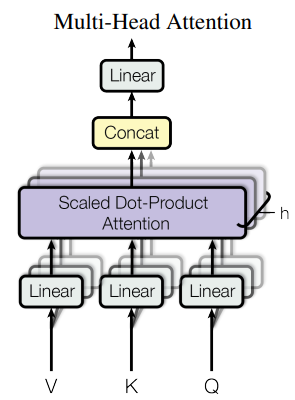
Multi-Head Attention은 Scaled Dot-Product Attention 여러 개를 Concat한 방법이다. 논문의 저자들은 하나의 Attention을 $d_{model}$ 차원의 query, key, value에 적용하는 것보다 서로 다르게 학습된 h번의 linear projection을 진하는 것이 효과적이라고 말한다. 이 때 Attention function은 병렬적으로 진행할 수 있고 $d_v$ 차원의 output을 만들어낸다.
$$ MultiHead(Q,K,V) = Concat(head_1, ..., head_h)W^O \\ \qquad \text{where} \; head_{i} = Attention(QW_{i}^{Q}, KW_{i}^{K}, VW_{i}^{V}) $$
1. (입력값 차원 수 / multihead 개수)의 차원으로 Q, K, V 생성
2. 각 Q, K, V를 h개의 버전으로 선형 변환
3. Q, K, V를 사용해 여러 버전의 Scaled Dot-Product Attention 진행
4. 각 버전을 concat
5. Concat한 값을 다시 한번 선형 변환
이 논문에서는 h = 8, $d_k$ = $d_v$ = $d_{model}/h$ = 64로 설정하였다. 각 head마다 차원을 줄이기 때문에 전체 computational cost는 하나의 Attention을 할 때와 비슷하다.
(3) Applications of Attention in our Model
Transformer는 3가지 방법으로 Multi-Head Attention을 사용한다.
1. Encoder-Decoder Attention layer
Decoder의 두 번째 sub-layer인 Multi-Head Attention layer에서는 Encoder의 output에서 key와 value를 받아온다. 이것은 Decoder의 모든 position에서 Input sequence의 모든 position을 고려할 수 있게 한다. (Query는 이전 Decoder layer에서 가져온다)
2. Encoder Self-Attention layer
key, value, query 모두 Encoder의 이전 layer에서 가져오고 Encoder의 각 position은 이전 layer의 모든 position을 고려한다.
3. Decoder Self-Attention layer
Decoder의 Self-Attention layer에서 각 position은 본인을 포함한 이전의 정보까지 참고(고려)할 수 있다. 이 때 모델의 Auto regressive 구조를 보존하기 위해 leftward information flow(뒤의 position의 정보를 참고하는 것)를 막아주어야 하는데, 논문에서는 이를 Scaled Dot-Product 과정에서 softmax를 들어가기전 illegal connection의 값들을 모두 $-\infty$로 masking 하는 방법으로 해결하였다. 이렇게 되면 softmax 연산시 해당 값들이 0에 가까운 값으로 나오게 되어 중요도가 떨어지게 된다.
Q1 : illegal connection? 현재 Position 뒤의 정보를 사용한 결과라고 생각되는데 왜 발생하는지?
Q2 : Encoder-Decoder Attention에서 왜 Encoder의 output 중 Key와 Value만을 받아오는 걸까?
3.3. Position-wise Feed-Forward Networks
$$ FFN(x) = max(0, xW_1 + b_1)W_2 + b_2$$
Encoder와 Decoder는 모두 Fully Connected Feed Forward Network를 거치는데, 이 때 각각의 position마다 동일하게 적용되기 때문에 Position-wise라고 부르며, 이 때 사용되는 2번의 선형 변환에는 ReLU함수를 사용한다.
Input, output size는 $d_{model} = 512$ 이고 inner-layer의 차원은 $d_{ff} = 2048$이다. FFN의 weight는 6개의 layer마다 다른 값으로 학습된다.
Q3 : 선형변환이 2번이라는 것은 hidden layer가 2개라는 의미인가?
3.4. Embeddings and Softmax
다른 Sequence Transduction 모델들처럼 input token과 output token을 $d_{model}$ 차원의 벡터로 변환하기 위해 학습된 Embedding을 사용하였다. 또한 2개의 Embedding layer와 softmax 전 선형 변환에서 같은 weight matrix를 공유한다. (Embedding layer에서는 weight들에 $\sqrt{d_{model}}$을 곱해준다)
Q4 : 2개의 Embedding layer라는 건 Input과 Output Embedding layer를 의미하는 것인가?
Q5 : 학습된 Embedding 이라는 건 뭔가?
3.5. Positional Encoding

Transformer 모델은 Recurrence나 Convolution을 사용하지 않았기 때문에 Sequence의 순서를 사용하기 위해 Sequence의 상대적이거나 절대적인 위치 정보를 넣어주어야 한다. 따라서 Encoder와 Decoder Stack의 아래에 Positional Encoding을 추가하여 Embedding Vector에 Positional Encoding 값을 더해준다. (Positional Encoding과 Input Embedding은 같은 차원을 가지기 때문에 더할 수 있음)

$$ PE(pos, 2i) = sin(pos/10000^{2i/d_{model}}) $$
$$ PE(pos, 2i+1) = cos(pos/10000^{2i/d_{model}}) $$
$pos$ : position ( 입력 문장에서 임베딩 벡터의 위치 )
$i$ : dimension ( 임베딩 계층 차원 인덱스 )
짝수 인덱스는 sine 함수, 홀수 인덱스는 cosine 함수를 이용해 위치를 나타낸다. 위 함수를 선택한 이유는 어떠한 offset k라도 $PE_{pos+k}$는 $PE_{pos}$의 선형 함수로 표현될 수 있어 학습이 쉬울 것이라고 생각했기 때문이다.
4. Why Self-Attention
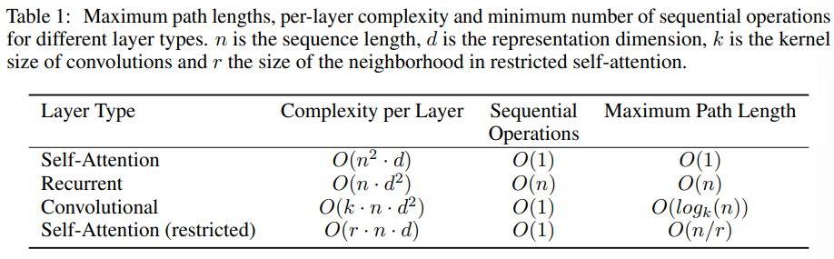
n : sequence length
d : representation Dimension (n<d)
k : kernel size of convolution
r : size of the neighborhood
※ Restricted Self-Attention
: 긴 sequence를 처리할 때의 복잡도를 낮추기 위해 해당 position의 neighborhood만 고려하는 방법
Recurrent / Convolutional 방법 대신 Self-Attention 방법을 선택한 이유
1. layer별 total computational complexity
2. 병렬화 할 수 있는 computation amount
3. Long-range Dependency 사이 path의 길이
Q6 : Maximum path의 길이가 왜 1인 건가?
<참고자료>
https://soki.tistory.com/m/108
https://wandukong.tistory.com/19
https://techblog-history-younghunjo1.tistory.com/497
https://kubig-2021-2.tistory.com/55
세 줄 요약
1. Attention Mechanism만을 이용해 RNN, CNN 구조를 대체하는 Transformer 아키텍처 제안
2. Self-Attention, Positional Encoding 등의 방법론을 사용하여 SOTA 성능을 달성
3. Encoder 구조만 사용한 BERT, Decoder 구조만 사용한 GPT, Vision Task에 사용하는 VIT 등 현재 NLP를 넘어 다양한 분야에 활용

'논문 paper 리뷰' 카테고리의 다른 글
| [Paper Review] Factorization Machines 논문 이해하기 (0) | 2023.04.09 |
|---|---|
| [Paper Review] Model Soup 논문 이해하기 (0) | 2023.03.19 |
| [X:AI] Inception-v2, v3논문 이해하기 (0) | 2023.03.16 |


댓글